In The System Shown Below The Two Continuous Time Signals
Holbox
Mar 12, 2025 · 6 min read
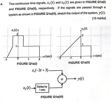
Table of Contents
Analyzing Continuous-Time Signals in a System: A Deep Dive
This article delves into the analysis of two continuous-time signals within a specified system. We'll explore various aspects, including signal representation, system response, convolution, and frequency domain analysis. Understanding these concepts is crucial for engineers and scientists working with signal processing, control systems, and numerous other fields. While a specific system diagram isn't provided in the prompt, we'll use generalized examples to illustrate the core principles.
Understanding Continuous-Time Signals
Continuous-time signals are functions whose domain is a continuous variable, usually representing time. Unlike discrete-time signals, which are defined only at discrete points in time, continuous-time signals have a value at every instant within a given interval. These signals are often represented mathematically by functions like:
- x(t): This denotes a continuous-time signal, where 't' represents time.
Several common types of continuous-time signals exist:
-
Sinusoidal Signals: These are periodic signals characterized by their amplitude, frequency, and phase. They form the building blocks for Fourier analysis. Example:
x(t) = A*sin(2πft + φ), where A is amplitude, f is frequency, and φ is phase. -
Exponential Signals: These signals exhibit exponential growth or decay. They are crucial in understanding system stability and transient responses. Example:
x(t) = Ae^(αt), where A is amplitude and α determines growth (α > 0) or decay (α < 0). -
Impulse Signals (Dirac Delta Function): The Dirac delta function, δ(t), is a generalized function representing an infinitely short pulse with unit area. It's invaluable in system analysis and convolution.
-
Step Signals (Unit Step Function): The unit step function, u(t), is defined as 0 for t < 0 and 1 for t ≥ 0. It's useful for modeling systems' responses to abrupt changes.
System Representation and Response
A system transforms an input signal into an output signal. Continuous-time systems are often represented using differential equations, transfer functions, or impulse responses.
-
Differential Equations: These equations describe the relationship between the input and output signals in the time domain. For example, a simple first-order system might be represented by:
dy(t)/dt + ay(t) = bx(t), where x(t) is the input, y(t) is the output, and 'a' and 'b' are system parameters. -
Transfer Functions: The transfer function, H(s), is the Laplace transform of the impulse response. It represents the system's frequency response and is a powerful tool for analyzing system stability and performance. The transfer function relates the Laplace transform of the input, X(s), to the Laplace transform of the output, Y(s):
Y(s) = H(s)X(s). -
Impulse Response, h(t): This is the system's output when the input is a Dirac delta function. It completely characterizes a linear time-invariant (LTI) system. The system's output, y(t), can be obtained by convolving the input signal, x(t), with the impulse response, h(t):
y(t) = x(t) * h(t).
Convolution: The Cornerstone of LTI System Analysis
Convolution is a mathematical operation that combines two signals to produce a third signal representing the system's output. For continuous-time signals, convolution is defined as:
y(t) = (x * h)(t) = ∫ x(τ)h(t - τ) dτ
where:
x(τ)is the input signal.h(t - τ)is the time-reversed and shifted impulse response.- The integral is taken over all values of τ.
Convolution represents the superposition of the system's response to each infinitesimal part of the input signal. It's a fundamental concept in signal processing because it allows us to determine the output of any LTI system given its impulse response and input signal. Convolution can be computationally intensive, but various techniques, including numerical methods and the Fast Fourier Transform (FFT), exist to speed up the process.
Frequency Domain Analysis: Fourier Transforms
The frequency domain provides a different perspective on signals and systems. The Fourier transform converts a signal from the time domain to the frequency domain, revealing its constituent frequencies and amplitudes. For continuous-time signals, the Fourier transform is defined as:
X(f) = ∫ x(t)e^(-j2πft) dt
where:
X(f)is the Fourier transform of x(t).fis the frequency.jis the imaginary unit.
The inverse Fourier transform converts a signal back from the frequency domain to the time domain:
x(t) = ∫ X(f)e^(j2πft) df
Frequency domain analysis is invaluable because it simplifies the analysis of LTI systems. The frequency response of a system, H(f), is the Fourier transform of its impulse response, h(t). In the frequency domain, the output spectrum, Y(f), is simply the product of the input spectrum, X(f), and the system's frequency response:
Y(f) = H(f)X(f)
This simplifies system analysis considerably, as multiplication in the frequency domain is equivalent to convolution in the time domain.
Analyzing the System with Two Continuous-Time Signals
To illustrate the concepts discussed above, let's consider a hypothetical system with two continuous-time input signals, x₁(t) and x₂(t), and an impulse response h(t). We'll analyze the system's behavior under various scenarios:
Scenario 1: Linear Superposition
If the system is linear, the response to the sum of two input signals is the sum of the individual responses. This is the principle of superposition:
y(t) = (x₁(t) + x₂(t)) * h(t) = x₁(t) * h(t) + x₂(t) * h(t)
Scenario 2: Different Input Signals
Consider two different input signals: x₁(t) = sin(2πt) (a sinusoidal signal) and x₂(t) = u(t) (a unit step signal). The system's response to each signal would differ depending on the system's characteristics. For example, if h(t) is a low-pass filter, the system would attenuate high-frequency components of x₁(t) and pass the low-frequency component of x₂(t) relatively unchanged.
Scenario 3: System with Feedback
Systems with feedback loops introduce additional complexity. The output of the system can influence the input, creating a closed-loop system. The analysis of such systems often involves techniques from control theory, such as block diagrams and transfer function manipulation.
Scenario 4: Non-Linear Systems
The principles outlined above apply primarily to linear time-invariant systems. Non-linear systems exhibit behaviors that don't obey the superposition principle. Their analysis often requires more complex methods, such as numerical simulation or Volterra series representation.
Practical Applications
The analysis of continuous-time signals and systems is vital across many fields, including:
- Signal Processing: Audio processing, image processing, communication systems.
- Control Systems: Design and analysis of control systems for various applications (robotics, aerospace, industrial automation).
- Communication Systems: Design of communication channels, modulation and demodulation techniques.
- Biomedical Engineering: Analysis of physiological signals (ECG, EEG), development of medical devices.
Conclusion
Understanding the behavior of continuous-time signals within a system is a cornerstone of many engineering and scientific disciplines. This involves mastering concepts such as signal representation, system response (differential equations, transfer functions, impulse responses), convolution, and frequency domain analysis (Fourier transforms). By applying these principles, we can effectively design, analyze, and optimize systems that process and manipulate continuous-time signals. This article provides a foundation for further exploration into the rich and diverse world of continuous-time signal processing. Remember to always consider the specifics of your system and the characteristics of your input signals when performing your analysis. The choice of analysis technique will depend heavily on the complexity of the system and the desired level of detail in the results.
Latest Posts
Latest Posts
-
Select All That Apply To Calcitonin
Mar 12, 2025
-
Draw The Major Product Of This Reaction Ignore Inorganic Byproducts
Mar 12, 2025
-
Meaningfulness Is Associated With Blank Rather Than Blank
Mar 12, 2025
-
Locking Out Tagging Out Refers To The Practice Of
Mar 12, 2025
-
What Is The Value Of The
Mar 12, 2025
Related Post
Thank you for visiting our website which covers about In The System Shown Below The Two Continuous Time Signals . We hope the information provided has been useful to you. Feel free to contact us if you have any questions or need further assistance. See you next time and don't miss to bookmark.
