Based On The Values In Cells A51 A55 What Formula
Holbox
Mar 26, 2025 · 6 min read
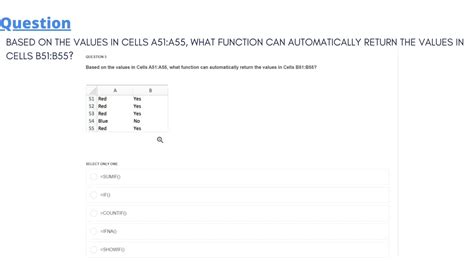
Table of Contents
- Based On The Values In Cells A51 A55 What Formula
- Table of Contents
- Based on the Values in Cells A51:A55, What Formula? A Deep Dive into Excel Formula Selection
- Understanding the Context: Data in A51:A55
- Common Excel Functions and Their Applications
- 1. Mathematical Functions
- 2. Text Functions
- 3. Date and Time Functions
- 4. Logical Functions
- 5. Lookup and Reference Functions
- Advanced Techniques and Formula Combinations
- Choosing the Right Formula: A Step-by-Step Approach
- Conclusion
- Latest Posts
- Latest Posts
- Related Post
Based on the Values in Cells A51:A55, What Formula? A Deep Dive into Excel Formula Selection
Choosing the right Excel formula is crucial for efficient data analysis and manipulation. This article delves into the process of selecting the appropriate formula based on the values contained within a specific cell range, such as A51:A55. We'll explore various scenarios, common functions, and advanced techniques to help you master formula selection in Excel.
Understanding the Context: Data in A51:A55
Before we discuss formulas, let's clarify the importance of understanding the data type and structure within cells A51:A55. The values in these cells will directly determine which formulas are applicable. Are the cells populated with:
- Numbers: This allows for mathematical operations (SUM, AVERAGE, MAX, MIN, etc.).
- Text: This necessitates text-based functions (CONCATENATE, LEFT, RIGHT, FIND, etc.).
- Dates: Date functions (YEAR, MONTH, DAY, TODAY, etc.) become essential.
- Boolean values (TRUE/FALSE): These are crucial for logical functions (IF, AND, OR, etc.).
- A mixture of data types: This often requires combining functions to handle different types appropriately.
Common Excel Functions and Their Applications
Let's explore some of the most frequently used Excel functions and how they apply to the data in A51:A55. Remember, the specific function you need will depend heavily on what you want to do with the data.
1. Mathematical Functions
If A51:A55 contains numerical data, the following functions are relevant:
-
SUM(A51:A55): This calculates the sum of all numbers in the specified range. This is perhaps the most common function for numerical data. It's incredibly versatile, particularly when combined with other functions.
-
AVERAGE(A51:A55): Calculates the average (mean) of the numbers in the range. Useful for understanding central tendency.
-
MAX(A51:A55): Returns the largest number in the range. Identifying maximum values is frequently necessary in data analysis.
-
MIN(A51:A55): Returns the smallest number in the range. The counterpart to MAX, helping to understand data range and outliers.
-
COUNT(A51:A55): Counts the number of cells containing numbers within the specified range. This differs from COUNTA.
-
COUNTA(A51:A55): Counts the number of cells that are not empty, regardless of data type.
2. Text Functions
If A51:A55 contains text data, you will need text functions:
-
CONCATENATE(A51,A52,A53,A54,A55): Joins the text from the cells into a single string. You can also use the ampersand (&) operator as a shorter alternative:
=A51&A52&A53&A54&A55 -
LEFT(A51,n): Extracts a specified number (n) of characters from the left side of the text string in A51.
-
RIGHT(A51,n): Extracts a specified number (n) of characters from the right side of the text string in A51.
-
MID(A51,start_num,num_chars): Extracts a specific number of characters from a text string, starting at a specified position.
-
FIND("text",A51): Locates the starting position of a specific text string within the text string in A51. Case-sensitive.
-
SEARCH("text",A51): Similar to FIND but not case-sensitive.
-
LEN(A51): Returns the number of characters in a text string.
3. Date and Time Functions
If A51:A55 contains dates, consider these:
-
YEAR(A51): Extracts the year from a date.
-
MONTH(A51): Extracts the month from a date.
-
DAY(A51): Extracts the day from a date.
-
TODAY(): Returns the current date.
-
NOW(): Returns the current date and time.
-
DATE(year,month,day): Creates a date value from separate year, month, and day values.
4. Logical Functions
Logical functions are essential for conditional calculations:
-
IF(logical_test,value_if_true,value_if_false): Performs a logical test and returns one value if the test is true and another if it's false. This is a fundamental building block of many complex Excel formulas.
-
AND(logical1, logical2,…): Returns TRUE only if all logical arguments are TRUE.
-
OR(logical1, logical2,…): Returns TRUE if at least one logical argument is TRUE.
-
NOT(logical): Reverses the logical value of an argument.
5. Lookup and Reference Functions
These functions are crucial for retrieving data from other parts of the spreadsheet:
-
VLOOKUP(lookup_value, table_array, col_index_num, [range_lookup]): Searches for a value in the first column of a table and returns a value in the same row from a specified column.
-
HLOOKUP(lookup_value, table_array, row_index_num, [range_lookup]): Similar to VLOOKUP, but searches across the first row.
-
INDEX(array, row_num, [col_num]): Returns a value from a range or array based on its row and column number.
-
MATCH(lookup_value, lookup_array, [match_type]): Finds the position of a value in a range or array. Often used in conjunction with INDEX.
Advanced Techniques and Formula Combinations
The power of Excel lies in combining multiple functions to perform complex calculations. Here are some examples based on data in A51:A55:
Example 1: Conditional Summation
Let's say you want to sum only the numbers in A51:A55 that are greater than 10. You can use SUMIF:
=SUMIF(A51:A55,">10")
Example 2: Counting Specific Text Strings
Suppose A51:A55 contains text, and you need to count how many cells contain the word "apple":
=COUNTIF(A51:A55,"apple")
Example 3: Combining Text and Numerical Data
Imagine A51:A53 contain numbers representing sales figures, and A54 contains the product name. You could create a summary like this:
="Total sales for "&A54&": "&SUM(A51:A53)
Example 4: Nested IF Statements
Nested IF statements allow for multiple conditional checks. For instance, assigning grades based on numerical scores in A51:A55:
=IF(A51>=90,"A",IF(A51>=80,"B",IF(A51>=70,"C","D"))) (This would need to be repeated for each cell A52-A55).
Example 5: Using INDEX and MATCH for Data Lookup
Suppose you have a separate table with product IDs in one column and prices in another. You could use INDEX and MATCH to look up the price of a product based on its ID in A51:A55:
(Assuming product IDs are in column B and prices in column C of another sheet named "Prices"):
=INDEX(Prices!C:C,MATCH(A51,Prices!B:B,0))
Choosing the Right Formula: A Step-by-Step Approach
-
Define your objective: Clearly state what you want to achieve with the formula. What calculation or manipulation are you trying to perform?
-
Analyze the data: Examine the data type and structure in A51:A55. Are they numbers, text, dates, or a mix?
-
Identify relevant functions: Based on your objective and data type, select the most appropriate Excel functions.
-
Test and refine: After constructing your formula, test it with a small sample of data to ensure accuracy. Refine as necessary.
-
Document your work: Add comments to your formulas to explain their purpose and functionality, especially when using complex combinations of functions. This will make it easier to understand and maintain your spreadsheet in the future.
Conclusion
Selecting the correct Excel formula is a critical skill for effective data analysis. By understanding the different function categories, combining functions effectively, and following a systematic approach, you can leverage the full power of Excel to manage and analyze your data efficiently. Remember to always clearly define your objectives and thoroughly test your formulas before relying on the results for decision-making. Mastering these techniques will significantly improve your productivity and analytical capabilities within Excel.
Latest Posts
Latest Posts
-
Which Of The Following Statements About Cycloaddition Reactions Is True
Mar 30, 2025
-
Elisa Graduated From College With A Double Major
Mar 30, 2025
-
The Inflation Rate Is Defined As The
Mar 30, 2025
-
Schedule Of Cost Of Goods Manufactured
Mar 30, 2025
-
Visceral Reflex Arcs Differ From Somatic In That
Mar 30, 2025
Related Post
Thank you for visiting our website which covers about Based On The Values In Cells A51 A55 What Formula . We hope the information provided has been useful to you. Feel free to contact us if you have any questions or need further assistance. See you next time and don't miss to bookmark.
