Using Cell References Enter A Formula In Cell B6
Holbox
Apr 01, 2025 · 6 min read
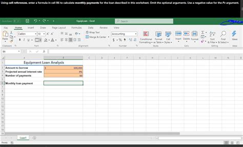
Table of Contents
- Using Cell References Enter A Formula In Cell B6
- Table of Contents
- Using Cell References to Enter Formulas in Cell B6: A Comprehensive Guide
- Understanding Cell References
- 1. Relative References
- 2. Absolute References
- 3. Mixed References
- Entering Formulas in Cell B6: Practical Examples
- 1. Simple Addition: Summing Values
- 2. Subtraction, Multiplication, and Division
- 3. Using Absolute References for Consistent Calculations
- 4. Combining Operations and Cell References
- 5. Referencing Cells Across Multiple Sheets
- 6. Using Functions with Cell References
- 7. Error Handling with IFERROR
- 8. Advanced Techniques: Array Formulas
- Best Practices for Using Cell References
- Conclusion
- Latest Posts
- Latest Posts
- Related Post
Using Cell References to Enter Formulas in Cell B6: A Comprehensive Guide
Entering formulas in spreadsheet software like Microsoft Excel or Google Sheets is fundamental to data manipulation and analysis. A core component of formula creation involves using cell references, which allow formulas to dynamically update based on changes in referenced cells. This comprehensive guide delves into the intricacies of using cell references to enter formulas in cell B6, exploring various scenarios and advanced techniques.
Understanding Cell References
Before diving into specific examples for cell B6, let's establish a foundational understanding of cell references. A cell reference is simply the address of a cell within a spreadsheet. It's expressed as a combination of a column letter and a row number. For example:
- A1: Refers to the cell in the first column (A) and first row (1).
- B10: Refers to the cell in the second column (B) and tenth row (10).
- Z100: Refers to the cell in the 26th column (Z) and 100th row.
There are three main types of cell references:
1. Relative References
These are the default type. When a formula with relative references is copied or moved, the references within the formula adjust relative to the new location. For instance, if a formula in A1 refers to B1, copying it to A2 will automatically change the reference to B2.
2. Absolute References
These references remain fixed regardless of where the formula is copied or moved. An absolute reference is denoted by a dollar sign ($) before either the column letter, the row number, or both.
- $A$1: Absolute reference to cell A1. This will always refer to cell A1, even when copied.
- $A1: Absolute column reference, relative row reference. The column will always be A, but the row will adjust when copied.
- A$1: Relative column reference, absolute row reference. The row will always be 1, but the column will adjust when copied.
3. Mixed References
These combine aspects of both relative and absolute references. They use dollar signs ($) strategically to lock either the column or the row, while the other remains relative. Examples include $A1 and A$1, as explained above.
Entering Formulas in Cell B6: Practical Examples
Now, let's explore various scenarios where you might enter formulas in cell B6 using different types of cell references. We'll assume your spreadsheet has data in columns A and C, possibly including numbers, text, or dates.
1. Simple Addition: Summing Values
Let's say you want to add the values in cells A1 and C1. The formula in B6 would be:
=A1+C1
This is a simple formula using relative references. If you copied this formula down to B7, it would automatically become =A2+C2, adding the values from the second row.
2. Subtraction, Multiplication, and Division
The same principles apply to other basic arithmetic operations:
- Subtraction:
=A1-C1(in B6) - Multiplication:
=A1*C1(in B6) - Division:
=A1/C1(in B6)
Remember, these are all relative references.
3. Using Absolute References for Consistent Calculations
Suppose you want to consistently add a fixed value (e.g., 10) from cell A1 to values in column C. You would use an absolute reference for cell A1:
=$A$1+C1 (in B6)
Copying this down would always add the value in A1 to the corresponding cell in column C.
4. Combining Operations and Cell References
You can combine multiple operations and cell references within a single formula. For instance, to calculate the average of cells A1, A2, and C1, and then subtract the value in C2:
=(A1+A2+C1)/3-C2 (in B6)
This demonstrates the flexibility of creating complex calculations using cell references.
5. Referencing Cells Across Multiple Sheets
If your data is spread across different sheets within the same workbook, you can still reference them in your formulas. To refer to a cell on a different sheet, precede the cell reference with the sheet name followed by an exclamation mark (!).
For example, if cell A1 on the "Sheet2" sheet contains a value you need to add to C1 on your current sheet, the formula in B6 would be:
=Sheet2!A1+C1
6. Using Functions with Cell References
Excel and Google Sheets offer numerous built-in functions that enhance your formula creation capabilities. These functions often require cell references as arguments.
-
SUM Function:
=SUM(A1:A10)sums the values in the range A1 to A10. You can adapt this to sum ranges relevant to your data in cell B6. For example,=SUM(A1:A5, C1:C5)sums the values in two different ranges. -
AVERAGE Function:
=AVERAGE(A1:C1)calculates the average of the values in cells A1, B1, and C1. -
COUNT Function:
=COUNT(A1:A10)counts the number of numeric values in the range A1 to A10. -
IF Function:
=IF(A1>10, "Greater than 10", "Less than or equal to 10")checks if the value in A1 is greater than 10 and returns different text accordingly. You can adapt this to use values from different cells, creating conditional logic. -
VLOOKUP and HLOOKUP Functions: These are powerful functions for retrieving data from a table based on a lookup value. They extensively use cell references to specify the lookup table and the column index.
-
INDEX and MATCH Functions: Often used together as a powerful alternative to VLOOKUP and HLOOKUP, providing more flexibility and efficiency. These functions also rely heavily on cell references.
7. Error Handling with IFERROR
Formulas can sometimes produce errors (e.g., #DIV/0! for division by zero, #REF! for invalid references). The IFERROR function allows you to handle these gracefully:
=IFERROR(A1/C1, 0)
This formula divides A1 by C1. If the division results in an error, it returns 0 instead of the error message. You can customize the second argument to return any alternative value or text.
8. Advanced Techniques: Array Formulas
Array formulas allow you to perform calculations on multiple cells simultaneously. These formulas are entered by pressing Ctrl + Shift + Enter (Windows) or Command + Shift + Return (Mac). The formula will be enclosed in curly braces {}.
For example, to sum the products of corresponding cells in two ranges:
{=SUM(A1:A5*C1:C5)}
Best Practices for Using Cell References
-
Clear Naming Conventions: Use descriptive names for your worksheets and cells (if possible) to improve formula readability and maintainability.
-
Careful Reference Selection: Double-check your cell references to avoid errors. Use the absolute or mixed references strategically.
-
Comments and Documentation: Add comments to your formulas, especially complex ones, to explain their logic and purpose. This is crucial for long-term understanding and maintenance of your spreadsheets.
-
Testing and Validation: After entering a formula, thoroughly test it with different data inputs to ensure it provides accurate results.
-
Data Validation: Implement data validation rules to prevent incorrect data entry and potential formula errors.
-
Regular Review: Periodically review your formulas to identify and correct any inaccuracies or inefficiencies.
Conclusion
Mastering the use of cell references is pivotal for effectively using spreadsheet software. This guide has explored a wide range of techniques, from basic arithmetic operations to advanced array formulas, covering different types of cell references and incorporating error handling and best practices. By applying these concepts, you can build powerful and robust spreadsheets capable of handling complex data analysis and manipulation tasks, all starting with a simple formula entered into cell B6. Remember, consistent practice and exploration will solidify your understanding and proficiency in this crucial aspect of spreadsheet functionality. Continue experimenting and expanding your knowledge to unlock the full potential of spreadsheet formulas.
Latest Posts
Latest Posts
-
According To The Efficient Market Hypothesis
Apr 05, 2025
-
Comparisons Of Financial Data Made Within A Company Are Called
Apr 05, 2025
-
The Components Of Global Market Assessment Include
Apr 05, 2025
-
Foundations For Teaching English Language Learners
Apr 05, 2025
-
Fraudulent Reporting By Management Could Include
Apr 05, 2025
Related Post
Thank you for visiting our website which covers about Using Cell References Enter A Formula In Cell B6 . We hope the information provided has been useful to you. Feel free to contact us if you have any questions or need further assistance. See you next time and don't miss to bookmark.
