The Matrix Below Represents A System Of Equations.
Holbox
Mar 20, 2025 · 6 min read
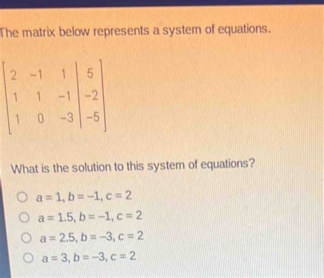
Table of Contents
Decoding the Matrix: A Deep Dive into Systems of Equations
Matrices are powerful tools in mathematics, offering a concise and elegant way to represent and solve systems of equations. This article will explore the intricacies of representing systems of equations using matrices, delve into various methods for solving these systems, and discuss the practical applications of this mathematical technique. We'll go beyond the basics, examining the nuances of different matrix types and their implications for solvability.
Understanding the Matrix Representation of Equations
A system of linear equations can be compactly represented using matrices. Let's consider a simple example:
- 2x + 3y = 7
- x - y = 1
This system can be represented using three matrices: a coefficient matrix, a variable matrix, and a constant matrix.
Coefficient Matrix (A): This matrix contains the coefficients of the variables in the equations. For our example:
A = | 2  3 |
    | 1 -1 |
Variable Matrix (X): This matrix contains the variables:
X = | x |
    | y |
Constant Matrix (B): This matrix contains the constants on the right-hand side of the equations:
B = | 7 |
    | 1 |
The system of equations can now be expressed in matrix form as: AX = B
This concise representation is crucial for applying various matrix operations to solve for the unknown variables (x and y).
Types of Matrices and Their Implications
The nature of the coefficient matrix significantly impacts the solvability of the system of equations. Let's examine some crucial matrix types:
-
Square Matrix: A square matrix has an equal number of rows and columns. This is a common scenario when the number of equations equals the number of variables. Square matrices can be further classified as singular (non-invertible) or non-singular (invertible). A non-singular matrix guarantees a unique solution to the system.
-
Rectangular Matrix: A rectangular matrix has an unequal number of rows and columns. This occurs when the number of equations differs from the number of variables. Such systems might have no solution, a unique solution, or infinitely many solutions.
-
Identity Matrix: An identity matrix (I) is a square matrix with 1s along the main diagonal and 0s elsewhere. It acts as a multiplicative identity, meaning that AI = IA = A.
-
Zero Matrix: A zero matrix is a matrix where all entries are zero. Multiplying any matrix by a zero matrix results in a zero matrix.
Methods for Solving Systems of Equations using Matrices
Several methods exist for solving systems of equations represented in matrix form. Let's explore some of the most prevalent:
1. Gaussian Elimination (Row Reduction)
Gaussian elimination is a fundamental method that involves transforming the augmented matrix [A|B] (formed by concatenating the coefficient and constant matrices) into row echelon form or reduced row echelon form through elementary row operations. These operations include:
- Swapping two rows: Interchanging the positions of two rows.
- Multiplying a row by a non-zero scalar: Multiplying all elements in a row by the same non-zero constant.
- Adding a multiple of one row to another: Adding a multiple of one row to another row.
By systematically applying these operations, the augmented matrix is simplified, revealing the solutions for the variables. Reduced row echelon form provides the solutions directly.
Example: Applying Gaussian elimination to our example system:
[A|B] = | 2  3 | 7 |
        | 1 -1 | 1 |
Through row operations, we can transform this into:
| 1  0 | 2 |
| 0  1 | 1 |
This indicates x = 2 and y = 1.
2. Inverse Matrix Method
If the coefficient matrix A is non-singular (invertible), the system AX = B can be solved by finding the inverse of A (denoted A⁻¹) and multiplying both sides by it:
A⁻¹AX = A⁻¹B
Since A⁻¹A = I (the identity matrix), this simplifies to:
IX = A⁻¹B or X = A⁻¹B
Calculating the inverse of a matrix can be computationally intensive, especially for larger matrices. Methods like the adjugate matrix method or using software tools are employed for this calculation.
3. Cramer's Rule
Cramer's rule is a method that uses determinants to solve for the variables. For a system of n equations with n variables, the solution for each variable xᵢ is given by:
xᵢ = det(Aᵢ) / det(A)
where det(A) is the determinant of the coefficient matrix A, and det(Aᵢ) is the determinant of the matrix formed by replacing the i-th column of A with the constant matrix B. Cramer's rule is elegant but computationally expensive for larger systems.
Applications of Matrix Representation and Solutions
The ability to represent and solve systems of equations using matrices has far-reaching applications across numerous fields:
-
Engineering: Solving complex systems of equations in structural analysis, circuit analysis, and control systems.
-
Computer Graphics: Representing transformations (rotation, scaling, translation) using matrices.
-
Economics: Modeling economic systems and analyzing input-output relationships.
-
Physics: Solving systems of equations in mechanics, electromagnetism, and quantum mechanics.
-
Machine Learning: Solving linear regression problems using matrix operations.
-
Cryptography: Employing matrices in encryption and decryption algorithms.
-
Operations Research: Optimizing resource allocation and scheduling using linear programming techniques, which heavily rely on matrix methods.
-
Data Science: Manipulating and analyzing large datasets effectively using matrix operations for tasks such as data transformation and dimensionality reduction.
Advanced Concepts and Challenges
While we've covered fundamental methods, solving large systems of equations presents computational challenges. The computational complexity of some methods increases significantly with the size of the matrix.
-
Numerical Stability: Rounding errors during computations can accumulate and affect the accuracy of the solutions, particularly for ill-conditioned matrices (matrices where small changes in the input lead to large changes in the output).
-
Iterative Methods: For very large systems, iterative methods like the Jacobi method or Gauss-Seidel method are preferred because they converge to the solution iteratively, reducing the computational burden of direct methods.
-
Singular Value Decomposition (SVD): SVD is a powerful technique used to analyze and solve systems of equations, particularly those with singular or ill-conditioned matrices. It helps in understanding the rank of the matrix and identifying the underlying structure of the system.
-
Sparse Matrices: Many real-world problems lead to sparse matrices (matrices with a high proportion of zero elements). Specialized algorithms are designed to exploit this sparsity, dramatically improving computational efficiency.
Conclusion
Matrices provide a robust and efficient framework for representing and solving systems of equations. Understanding the different types of matrices, the various solution methods, and the potential computational challenges is crucial for effectively applying these techniques across a wide range of applications. As we've seen, from the straightforward Gaussian elimination to the more sophisticated SVD, the choice of method depends on the specific characteristics of the system and the desired level of accuracy. Mastering these concepts empowers you to tackle complex problems and gain deeper insights into mathematical modeling across diverse fields. The beauty of matrix algebra lies in its ability to encapsulate complex relationships in a compact and manageable format, leading to elegant solutions and a better understanding of the underlying systems.
Latest Posts
Latest Posts
-
The Great Compromise Did All Of The Following Except
Mar 20, 2025
-
Altering The Three Dimensional Structure Of An Enzyme Might
Mar 20, 2025
-
According To Ich E6 An Audit Is Defined As
Mar 20, 2025
-
Which Is Not A Strategy For Defusing Potentially Harmful Situations
Mar 20, 2025
-
Write The Ions Present In A Solution Of Na3po4
Mar 20, 2025
Related Post
Thank you for visiting our website which covers about The Matrix Below Represents A System Of Equations. . We hope the information provided has been useful to you. Feel free to contact us if you have any questions or need further assistance. See you next time and don't miss to bookmark.
