The General Model For Calculating A Quantity Variance Is
Holbox
Mar 17, 2025 · 6 min read
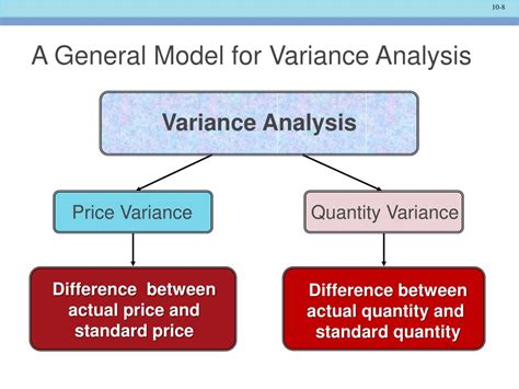
Table of Contents
The General Model for Calculating a Quantity Variance: A Deep Dive
Understanding and effectively calculating quantity variances is crucial for businesses seeking to optimize their operations and enhance profitability. This comprehensive guide delves into the general model for calculating quantity variances, exploring its various applications, interpretations, and the crucial role it plays in cost control and performance analysis. We'll cover everything from the fundamental formula to advanced scenarios, providing you with a complete understanding of this critical management accounting concept.
What is a Quantity Variance?
A quantity variance measures the difference between the actual quantity of materials or labor used in production and the standard or budgeted quantity that should have been used, given the actual output achieved. It helps pinpoint inefficiencies in resource utilization, whether due to waste, spoilage, theft, or simply poor production planning. This variance is expressed in monetary terms, making it readily comparable to other financial metrics and facilitating effective decision-making.
The significance of understanding quantity variance extends beyond simple cost analysis. It offers valuable insights into operational processes, revealing areas requiring improvement and facilitating the implementation of corrective actions to enhance overall efficiency and reduce costs. By pinpointing inefficiencies, businesses can target specific areas for optimization, leading to improved profitability and sustained growth.
The General Formula for Calculating Quantity Variance
The basic formula for calculating a quantity variance is deceptively simple, yet its implications are far-reaching:
Quantity Variance = (Actual Quantity - Standard Quantity) x Standard Price/Rate
Let's break down each component:
-
Actual Quantity: This refers to the actual amount of materials or labor hours consumed during the production process. This is a verifiable figure derived from production records.
-
Standard Quantity: This is the amount of materials or labor hours that should have been used to produce the actual output, based on pre-determined standards or budgets. This is usually calculated using predetermined standards like standard usage per unit of output multiplied by the actual units produced.
-
Standard Price/Rate: This is the predetermined cost per unit of material or labor hour. It reflects the expected cost based on market prices, historical data, or other relevant factors.
Note: The sign of the quantity variance is critical. A positive variance indicates that more resources were used than planned (an unfavorable variance, often denoted as U), while a negative variance signifies that fewer resources were used than planned (a favorable variance, often denoted as F).
Applying the Formula: Different Scenarios and Interpretations
The calculation of quantity variance remains consistent across various scenarios, but the interpretation can vary depending on the specific context. Let's examine a few common scenarios:
Scenario 1: Material Quantity Variance
Imagine a bakery producing loaves of bread. The standard quantity of flour required for each loaf is 500 grams, and the standard price of flour is $0.10 per gram. In a given week, the bakery produced 1000 loaves of bread and used 550,000 grams of flour.
Calculation:
- Actual Quantity = 550,000 grams
- Standard Quantity = 1000 loaves * 500 grams/loaf = 500,000 grams
- Standard Price = $0.10/gram
Quantity Variance = (550,000 - 500,000) * $0.10 = $5,000 (Unfavorable)
Interpretation: The bakery used 50,000 grams more flour than expected, resulting in a $5,000 unfavorable material quantity variance. This could be due to waste, spoilage, inefficient mixing processes, or inaccurate measuring.
Scenario 2: Labor Quantity Variance
A manufacturing company produces widgets. The standard labor hours per widget are 2 hours, and the standard labor rate is $25 per hour. During the month, the company produced 1000 widgets and used 2200 labor hours.
Calculation:
- Actual Quantity = 2200 labor hours
- Standard Quantity = 1000 widgets * 2 hours/widget = 2000 labor hours
- Standard Rate = $25/hour
Quantity Variance = (2200 - 2000) * $25 = $5,000 (Unfavorable)
Interpretation: The company used 200 more labor hours than expected, resulting in a $5,000 unfavorable labor quantity variance. This could be due to inexperienced workers, inefficient production processes, machine breakdowns requiring more manual intervention, or unforeseen delays.
Scenario 3: Investigating the Root Cause of a Variance
Identifying the cause of a variance is as crucial as calculating it. A significant unfavorable variance requires a thorough investigation. Possible causes include:
- Poor quality materials: Leading to increased wastage and rework.
- Inefficient equipment: Causing slower production rates and increased resource consumption.
- Lack of training: Resulting in unskilled labor and increased labor hours.
- Poor work planning: Leading to inefficiencies and excessive resource utilization.
- Inadequate supervision: Allowing wastage and unnecessary expenses.
- Theft or pilferage: Directly impacting material usage.
- Changes in product design: Requiring more material than previously anticipated.
Beyond the Basic Formula: Advanced Considerations
While the basic formula provides a solid foundation, several factors can influence the accuracy and interpretation of quantity variances:
-
Multiple Materials: For products requiring multiple materials, a separate quantity variance is calculated for each material. The total material quantity variance is the sum of individual variances.
-
Mixed Variance: Quantity variances are often analyzed in conjunction with price variances to provide a holistic view of cost overruns or undershoots. This combined analysis reveals whether the cost increase is predominantly due to higher prices or increased quantities.
-
Statistical Process Control (SPC): SPC techniques can be integrated into quantity variance analysis to identify patterns and trends in resource utilization, allowing for proactive interventions and preventive measures.
Using Quantity Variances for Continuous Improvement
The ultimate goal of calculating quantity variances isn't just to identify problems; it's to leverage that information to improve operational efficiency. Here's how:
-
Benchmarking: Comparing your quantity variances to industry benchmarks can reveal areas where your performance lags behind competitors.
-
Root Cause Analysis: As mentioned earlier, identifying the root cause of unfavorable variances is crucial for implementing effective corrective actions. Tools like the "5 Whys" technique can be helpful in this process.
-
Process Improvement Initiatives: Unfavorable variances often indicate the need for process improvements such as streamlining production workflows, investing in new equipment, or implementing better training programs.
-
Performance Evaluation: Quantity variances can be used to evaluate the performance of production managers and workers, incentivizing them to minimize waste and improve efficiency.
-
Budgeting and Forecasting: Accurate quantity variances can enhance the accuracy of future budgets and forecasts, enabling more informed decision-making.
Conclusion: Quantity Variance – A Powerful Tool for Operational Excellence
The general model for calculating quantity variances is a fundamental tool for cost control and operational efficiency. By systematically tracking and analyzing these variances, businesses can identify areas for improvement, reduce waste, and enhance overall profitability. Remember, the process is not merely about calculating numbers; it's about using those numbers to drive continuous improvement and achieve operational excellence. The insightful interpretation and application of quantity variance analysis ultimately contribute to a stronger bottom line and a more robust competitive position in the marketplace. Regular monitoring and proactive management of quantity variances are key elements in creating a lean, efficient, and profitable organization.
Latest Posts
Latest Posts
-
What Are The Effects Of Unanticipated Deflation
Mar 17, 2025
-
How To Cite Surveys In Mla
Mar 17, 2025
-
Wordpress Is Popular Free And Open Source
Mar 17, 2025
-
The Difference Between Aerobic And Anaerobic Glucose Breakdown Is
Mar 17, 2025
-
On December 29 2020 Patel Products
Mar 17, 2025
Related Post
Thank you for visiting our website which covers about The General Model For Calculating A Quantity Variance Is . We hope the information provided has been useful to you. Feel free to contact us if you have any questions or need further assistance. See you next time and don't miss to bookmark.
