Solve The Recurrence In Asymptotically Tight Big Oh Function:
Holbox
Mar 10, 2025 · 6 min read
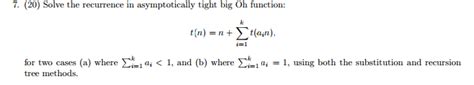
Table of Contents
Solving Recurrences in Asymptotically Tight Big O Notation
Understanding how to solve recurrence relations is crucial for analyzing the time and space complexity of algorithms. This is because many algorithms' performance can be modeled using recursive relationships, where the execution time depends on the execution time of smaller subproblems. Expressing this complexity using Big O notation provides a concise and robust way to compare algorithm efficiency. This article will delve deep into solving recurrences and expressing their solutions in asymptotically tight Big O notation. We'll explore various techniques, including the Master Theorem, substitution method, recursion tree method, and the iterative method.
Understanding Recurrence Relations
A recurrence relation defines a sequence where each term is a function of the preceding terms. In algorithm analysis, these terms typically represent the time or space required to solve a problem of a given size. A general form of a recurrence relation looks like this:
T(n) = aT(n/b) + f(n)
Where:
- T(n): Represents the time complexity of the problem of size 'n'.
- a: The number of subproblems in the recursive call.
- n/b: The size of each subproblem.
- f(n): The time complexity of the work done outside the recursive calls (e.g., dividing the problem, combining subproblem solutions).
Methods for Solving Recurrences
Several methods exist for solving recurrence relations. The choice of method depends on the specific form of the recurrence.
1. The Master Theorem
The Master Theorem provides a direct solution for many divide-and-conquer recurrences. It's a powerful tool when applicable, offering a quick and efficient solution. The theorem states:
Given a recurrence of the form T(n) = aT(n/b) + f(n), where a ≥ 1, b > 1, and f(n) is an asymptotically positive function:
-
Case 1: If f(n) = O(n<sup>log<sub>b</sub>a - ε</sup>) for some constant ε > 0, then T(n) = Θ(n<sup>log<sub>b</sub>a</sup>). This means the time complexity is dominated by the recursive calls.
-
Case 2: If f(n) = Θ(n<sup>log<sub>b</sub>a</sup>), then T(n) = Θ(n<sup>log<sub>b</sub>a</sup> log n). The time complexity is dominated by both the recursive calls and the work done outside them.
-
Case 3: If f(n) = Ω(n<sup>log<sub>b</sub>a + ε</sup>) for some constant ε > 0, and if af(n/b) ≤ cf(n) for some constant c < 1 and sufficiently large n, then T(n) = Θ(f(n)). The time complexity is dominated by the work done outside the recursive calls.
Example:
Consider the recurrence T(n) = 9T(n/3) + n. Here, a = 9, b = 3, and f(n) = n.
log<sub>b</sub>a = log<sub>3</sub>9 = 2.
Since f(n) = n = Θ(n<sup>2</sup>), we are in Case 2 of the Master Theorem. Therefore, T(n) = Θ(n<sup>2</sup> log n).
2. Substitution Method
The substitution method involves making a guess about the solution and then proving it using mathematical induction. This method requires careful consideration and often involves intricate calculations.
Steps:
-
Guess: Make an educated guess about the solution's form (e.g., O(n<sup>2</sup>), O(n log n)).
-
Induction Base Case: Prove the base case for small values of n (e.g., n = 1, 2).
-
Inductive Hypothesis: Assume the guess holds true for values smaller than n.
-
Inductive Step: Substitute the inductive hypothesis into the recurrence relation and show that the guess also holds true for n.
Example:
Let's solve T(n) = T(n-1) + n using the substitution method. We guess T(n) = O(n<sup>2</sup>). Let's assume T(k) ≤ ck<sup>2</sup> for some constant c and all k < n. Then:
T(n) = T(n-1) + n ≤ c(n-1)<sup>2</sup> + n = cn<sup>2</sup> - 2cn + c + n
To prove this is less than or equal to cn<sup>2</sup>, we need:
cn<sup>2</sup> - 2cn + c + n ≤ cn<sup>2</sup>
-2cn + c + n ≤ 0
This inequality holds for sufficiently large n if we choose an appropriate constant c. Therefore, our guess T(n) = O(n<sup>2</sup>) is correct.
3. Recursion Tree Method
The recursion tree method visualizes the recursive calls as a tree. Each node represents a subproblem, and the work done at each level is summed. This method is particularly helpful for understanding the contribution of different parts of the recurrence.
Steps:
-
Draw the tree: Represent each recursive call as a node.
-
Cost at each level: Calculate the work done at each level of the tree.
-
Sum the costs: Sum the costs of all levels to get the total cost.
-
Analyze the sum: Express the total cost using Big O notation.
Example:
Consider T(n) = 2T(n/2) + n.
The tree would show a branching factor of 2, with each subproblem size halved at each level. The cost at each level would be 'n'. The number of levels would be log<sub>2</sub>n. Therefore, the total cost is approximately n log<sub>2</sub>n, so T(n) = O(n log n).
4. Iterative Method
The iterative method involves repeatedly expanding the recurrence until a pattern emerges. This pattern can then be used to derive a closed-form solution. This is often the most straightforward approach for simple recurrences.
Example:
Let's solve T(n) = T(n-1) + 1 with T(1) = 1.
T(n) = T(n-1) + 1 T(n-1) = T(n-2) + 1 ... T(2) = T(1) + 1
Substituting repeatedly:
T(n) = T(1) + (n-1) = 1 + (n-1) = n
Therefore, T(n) = O(n).
Choosing the Right Method
The choice of the best method depends on the specific recurrence relation.
-
Master Theorem: Ideal for divide-and-conquer recurrences fitting its specific criteria.
-
Substitution Method: Requires a good initial guess, but provides a rigorous proof.
-
Recursion Tree Method: Offers good intuition and visualization, especially for understanding the structure of the recurrence.
-
Iterative Method: Simple and straightforward for relatively simple recurrences.
Advanced Considerations and Variations
This discussion primarily focuses on common types of recurrence relations. However, more complex scenarios exist:
-
Non-linear recurrences: These involve non-linear relationships between terms, making analysis more challenging. Approximation techniques often become necessary.
-
Recurrences with multiple variables: These arise in multi-dimensional problems and require more advanced techniques to solve.
-
Recurrences with floor and ceiling functions: The presence of floor and ceiling functions can complicate the analysis, requiring careful consideration of boundary conditions.
Conclusion
Solving recurrence relations is a fundamental skill for algorithm analysis. Mastering the techniques outlined above—the Master Theorem, substitution method, recursion tree method, and iterative method—equips you to analyze the time and space complexity of various algorithms effectively. Choosing the appropriate method depends on the form of the recurrence and your comfort level with each technique. Remember that the goal is not just to find a solution, but to find an asymptotically tight solution expressed using Big O notation, giving a precise representation of the algorithm's performance as the input size grows. Consistent practice and a solid understanding of these methods are key to achieving proficiency in this crucial area of computer science.
Latest Posts
Latest Posts
-
Documenting The Gba Plus Process Can Assist You With
Mar 10, 2025
-
What Is A Homonym For Soar
Mar 10, 2025
-
A Cashier Is Finishing A Transaction With A Customer
Mar 10, 2025
-
Hey Mom I Finished That Book About Jennifer
Mar 10, 2025
-
Documents Are Marked With A Number And Then A Name
Mar 10, 2025
Related Post
Thank you for visiting our website which covers about Solve The Recurrence In Asymptotically Tight Big Oh Function: . We hope the information provided has been useful to you. Feel free to contact us if you have any questions or need further assistance. See you next time and don't miss to bookmark.
