Determine F12 And F21 For The Following Configurations
Holbox
Mar 30, 2025 · 6 min read
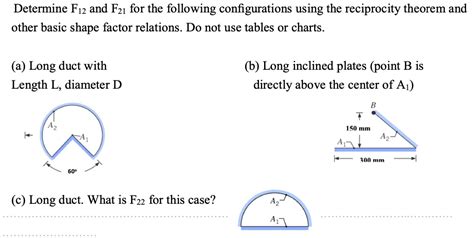
Table of Contents
- Determine F12 And F21 For The Following Configurations
- Table of Contents
- Determining F12 and F21: A Comprehensive Guide to Configuration-Specific Calculations
- Understanding F12 and F21
- Determining F12 and F21: Different Scenarios and Approaches
- Scenario 1: Simple Two-State System with Experimental Kinetic Data
- Scenario 2: Equilibrium Constant and One Rate Constant Known
- Scenario 3: Complex Multi-State System with Detailed Balance
- Scenario 4: Transition State Theory (TST)
- Scenario 5: Simulation Methods (Molecular Dynamics and Monte Carlo)
- Data Analysis and Considerations
- Conclusion
- Latest Posts
- Latest Posts
- Related Post
Determining F12 and F21: A Comprehensive Guide to Configuration-Specific Calculations
Determining the forward and reverse rate constants, F12 and F21, is a crucial aspect of understanding and modeling various dynamic systems. These constants represent the transition rates between two states, 1 and 2, often in chemical kinetics, population dynamics, or other fields involving state transitions. The exact method for determining F12 and F21 depends heavily on the specific configuration of the system and the available data. This article provides a comprehensive overview of various scenarios and approaches to tackling this problem.
Understanding F12 and F21
Before diving into specific methods, let's clarify the meaning of F12 and F21:
-
F12: This represents the forward rate constant, signifying the rate at which the system transitions from state 1 to state 2. It's often expressed as the probability of transition per unit time.
-
F21: This is the reverse rate constant, indicating the rate of transition from state 2 back to state 1. Similar to F12, it represents a probability per unit time.
The ratio of F12 and F21 is often related to the equilibrium constant (K) of the system, where K = F12/F21 at equilibrium. This relationship is fundamental in many applications.
Determining F12 and F21: Different Scenarios and Approaches
The methods for determining F12 and F21 vary greatly depending on the nature of the data and the system under consideration. Here are several common scenarios and associated approaches:
Scenario 1: Simple Two-State System with Experimental Kinetic Data
If you have experimental data tracing the concentration or population of states 1 and 2 over time, you can use kinetic modeling techniques. This often involves fitting the data to a set of differential equations that describe the system's dynamics.
Method:
-
Differential Equations: For a simple two-state system, the rate equations are:
d[1]/dt = -F12[1] + F21[2] d[2]/dt = F12[1] - F21[2]
where [1] and [2] represent the concentrations or populations of state 1 and state 2, respectively.
-
Data Fitting: Utilize non-linear regression techniques (e.g., least-squares fitting) to fit the experimental data to these differential equations. The fitting process will estimate the values of F12 and F21 that best match the observed kinetics. Software packages like MATLAB, Python (with SciPy), or specialized kinetics software are commonly employed for this purpose.
-
Model Validation: After fitting, it's crucial to validate the model. Check the goodness of fit (e.g., R-squared value) and ensure the model accurately predicts the behavior of the system under different conditions.
Example: Consider a chemical reaction A <=> B. By monitoring the concentrations of A and B over time and fitting the data to the above equations, you can determine the rate constants for the forward (A to B) and reverse (B to A) reactions.
Scenario 2: Equilibrium Constant and One Rate Constant Known
If you know the equilibrium constant (K) and one of the rate constants (either F12 or F21), you can easily calculate the other.
Method:
-
Equilibrium Relationship: Recall that K = F12/F21 at equilibrium.
-
Calculation: If you know K and F12, then F21 = F12/K. Similarly, if you know K and F21, then F12 = K * F21.
This scenario is particularly useful when one rate constant can be determined independently (e.g., through a separate experiment) or through theoretical considerations.
Scenario 3: Complex Multi-State System with Detailed Balance
In more complex scenarios with multiple interacting states, the principle of detailed balance can be a powerful tool. Detailed balance implies that at equilibrium, the flux between any two states must be equal in both directions.
Method:
-
Microscopic Reversibility: Detailed balance relies on the concept of microscopic reversibility, which assumes that at equilibrium, each elementary step and its reverse occur with equal probability.
-
Flux Balance: For each pair of states (i, j), the flux from i to j (Fi,j) must equal the flux from j to i (Fj,i) at equilibrium. This provides a system of equations that can be solved to determine the rate constants.
-
Solving the System: This often involves solving a system of non-linear equations, which can be computationally intensive for large systems.
This approach is particularly useful when the system's energy landscape is known, allowing the calculation of equilibrium populations and the application of detailed balance.
Scenario 4: Transition State Theory (TST)
For systems where the transition states between states 1 and 2 are well-defined, transition state theory (TST) can be used to estimate the rate constants.
Method:
-
Potential Energy Surface: TST requires knowledge of the potential energy surface of the system. This surface describes the energy landscape of the system, including the energies of the reactants, products, and the transition state.
-
Partition Functions: TST utilizes partition functions (statistical mechanics concepts) to calculate the rate constants. These partition functions depend on the properties of the reactants, products, and the transition state.
-
Rate Constant Calculation: The rate constants (F12 and F21) are then estimated using formulas derived from TST, which typically involve the activation energy (energy difference between the reactant and transition state) and the temperature.
TST is a powerful tool for estimating rate constants but requires detailed information about the potential energy surface and the properties of the involved species.
Scenario 5: Simulation Methods (Molecular Dynamics and Monte Carlo)
For complex systems where analytical solutions are intractable, computational methods like molecular dynamics (MD) and Monte Carlo (MC) simulations can be employed.
Method:
-
Simulation Setup: Create a computational model of the system, specifying the interactions between the constituent particles or components.
-
Simulation Run: Perform the simulation for sufficient time to allow the system to reach equilibrium or to observe the transitions between states 1 and 2.
-
Rate Constant Estimation: The rate constants are then estimated from the simulation trajectories by analyzing the frequency of transitions between states.
These methods are computationally expensive but are invaluable when experimental or analytical approaches are not feasible.
Data Analysis and Considerations
Regardless of the chosen method, careful data analysis is essential:
-
Error Analysis: Quantify the uncertainties in the estimated rate constants, accounting for experimental errors, fitting uncertainties, and other sources of variability.
-
Sensitivity Analysis: Evaluate the sensitivity of the estimated rate constants to changes in the input parameters or assumptions.
-
Model Validation: Thoroughly validate the chosen model by comparing its predictions to independent experimental data or observations.
Conclusion
Determining F12 and F21 requires a tailored approach dependent on the specific configuration of the system and the available data. This article outlined several common scenarios and associated methodologies, encompassing experimental kinetic analysis, equilibrium considerations, detailed balance, transition state theory, and computational simulation techniques. Remember to always carefully consider error analysis, sensitivity analysis, and model validation to ensure the reliability and accuracy of the results. The choice of method will ultimately be guided by the complexity of the system, the available resources, and the desired level of accuracy. This multifaceted approach to determining these crucial rate constants underscores the importance of a thorough understanding of both theoretical principles and practical data analysis techniques.
Latest Posts
Latest Posts
-
Reference Cell A1 From Alpha Worksheet
Apr 02, 2025
-
Professional Practice Use Of The Theories Concepts Presented In The Article
Apr 02, 2025
-
Ordinary Repairs And Maintenance Costs Should Be
Apr 02, 2025
-
Trina Is Trying To Decide Which Lunch Combination
Apr 02, 2025
-
Which Statement Best Describes A Command Economy
Apr 02, 2025
Related Post
Thank you for visiting our website which covers about Determine F12 And F21 For The Following Configurations . We hope the information provided has been useful to you. Feel free to contact us if you have any questions or need further assistance. See you next time and don't miss to bookmark.
