A Set Of Bivariate Data Was Used To Create
Holbox
Mar 18, 2025 · 6 min read
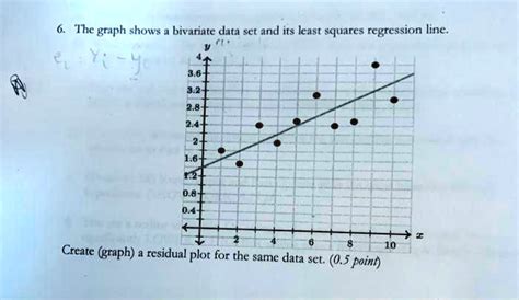
Table of Contents
Unveiling Insights: A Deep Dive into Bivariate Data Analysis
Bivariate data analysis is a cornerstone of statistical investigation, allowing us to explore the relationship between two variables. Understanding this relationship is crucial across numerous fields, from economics and finance to healthcare and environmental science. This comprehensive guide delves into the multifaceted world of bivariate data analysis, exploring its methods, interpretations, and practical applications. We'll move beyond simple definitions to uncover the nuances and power inherent in this analytical approach.
What is Bivariate Data?
Bivariate data refers to a dataset comprising observations on two variables for each individual or unit in the sample. These variables can be of different types:
- Quantitative: Numerical data representing measurements or counts (e.g., height, weight, income, temperature).
- Qualitative (Categorical): Data representing categories or groups (e.g., gender, eye color, type of car).
The nature of the variables dictates the appropriate analytical techniques. For instance, analyzing the relationship between height (quantitative) and weight (quantitative) differs significantly from analyzing the relationship between gender (categorical) and smoking status (categorical).
Methods for Analyzing Bivariate Data
The choice of analytical method hinges on the types of variables involved. Let's examine the key techniques:
1. Scatter Plots (for two quantitative variables):
Scatter plots are a visual representation of the relationship between two quantitative variables. Each point on the plot represents a single observation, with its horizontal position determined by one variable and its vertical position determined by the other. Scatter plots effectively reveal:
- Direction of the relationship: A positive relationship (as one variable increases, the other increases), a negative relationship (as one variable increases, the other decreases), or no apparent relationship.
- Strength of the relationship: The closer the points cluster around a line, the stronger the relationship. Scattered points indicate a weak relationship.
- Presence of outliers: Points significantly distant from the overall pattern may be outliers, warranting further investigation.
Example: A scatter plot showing the relationship between hours studied and exam scores would reveal if increased study time correlates with higher scores.
2. Correlation Coefficient (for two quantitative variables):
The correlation coefficient (often denoted as 'r') is a numerical measure quantifying the linear relationship between two quantitative variables. It ranges from -1 to +1:
- r = +1: Perfect positive linear correlation.
- r = 0: No linear correlation.
- r = -1: Perfect negative linear correlation.
Important Note: Correlation does not imply causation. A strong correlation merely suggests an association; it does not prove that one variable causes changes in the other.
3. Contingency Tables (for two categorical variables):
Contingency tables (also known as cross-tabulation tables) display the frequency distribution of two categorical variables. They show the number of observations falling into each combination of categories. From a contingency table, we can calculate:
- Conditional probabilities: The probability of one event given that another event has occurred.
- Relative frequencies: The proportion of observations in each cell relative to the total number of observations.
- Chi-square test: A statistical test to determine if there is a significant association between the two categorical variables.
Example: A contingency table could show the relationship between gender (male/female) and smoking status (smoker/non-smoker).
4. Regression Analysis (for two quantitative variables):
Regression analysis aims to model the relationship between a dependent variable (the outcome) and one or more independent variables (predictors). In bivariate regression, we have only one independent variable. The most common type is linear regression, which assumes a linear relationship between the variables. The output includes:
- Regression equation: A mathematical formula describing the relationship (e.g., Y = a + bX).
- R-squared: A measure of the goodness of fit of the model, indicating the proportion of variance in the dependent variable explained by the independent variable.
- Coefficients (a and b): The intercept (a) and slope (b) of the regression line.
Example: Predicting house prices (dependent variable) based on house size (independent variable).
5. Spearman's Rank Correlation (for two ordinal or quantitative variables):
Spearman's rank correlation measures the monotonic relationship between two variables. Monotonic means that as one variable increases, the other tends to increase or decrease, but not necessarily linearly. This is particularly useful when:
- The data are ordinal (ranked data).
- The relationship is not linear.
Interpreting Results and Drawing Conclusions
Analyzing bivariate data is not just about calculating statistics; it's about interpreting the findings within the context of the research question. Key considerations include:
- Statistical significance: Determining if the observed relationship is likely due to chance or represents a real effect. P-values and confidence intervals provide insights into significance.
- Effect size: The magnitude of the relationship between the variables. A statistically significant relationship might have a small effect size, indicating limited practical importance.
- Causation vs. Correlation: Always emphasize that correlation does not imply causation. Other factors might be influencing the observed relationship.
- Limitations of the data: Acknowledge any limitations of the data, such as sampling bias or measurement error, that could affect the conclusions.
Practical Applications of Bivariate Data Analysis
The applications are vast and span diverse fields:
- Economics: Analyzing the relationship between inflation and unemployment, consumer spending and income.
- Finance: Examining the correlation between stock prices and interest rates, risk and return.
- Healthcare: Investigating the association between lifestyle factors (e.g., diet, exercise) and health outcomes (e.g., heart disease, diabetes).
- Environmental Science: Studying the relationship between pollution levels and respiratory illnesses, temperature and sea level.
- Marketing: Analyzing the effectiveness of advertising campaigns by examining the relationship between advertising spend and sales.
- Education: Exploring the relationship between study habits and academic performance, teaching methods and student engagement.
Choosing the Right Method: A Summary
The selection of the appropriate analytical technique depends entirely on the nature of the two variables:
| Variable Type | Method | Description |
|---|---|---|
| Quantitative, Quantitative | Scatter Plot, Correlation, Regression | Visualize the relationship, quantify linear association, model the relationship |
| Categorical, Categorical | Contingency Table, Chi-square Test | Examine frequencies, test for association |
| Quantitative, Ordinal or vice versa | Spearman's Rank Correlation | Measure monotonic relationship |
Beyond Bivariate Analysis: Extending the Scope
While bivariate analysis provides valuable insights, it's often beneficial to extend the analysis to consider more than two variables. Multivariate analysis techniques, such as multiple regression, ANOVA, and MANOVA, allow for a more comprehensive understanding of complex relationships. These techniques are crucial when dealing with situations where multiple factors influence the outcome variable.
Conclusion
Bivariate data analysis is a fundamental tool for uncovering patterns and relationships within datasets. By carefully selecting the appropriate method and interpreting the results in context, researchers can draw valuable conclusions and make informed decisions across a wide range of disciplines. Remember to always consider the limitations of the data and avoid drawing causal inferences from correlations alone. Mastering bivariate data analysis is an essential skill for anyone involved in data-driven decision-making. Through careful consideration of the data type and the chosen analysis method, powerful insights can be uncovered, leading to a deeper understanding of the phenomena under investigation. This understanding, in turn, can inform better decision-making across a multitude of fields. The journey from raw data to meaningful conclusions requires careful planning, appropriate methodology, and a critical approach to interpretation.
Latest Posts
Latest Posts
-
The Most Common Output Device For Soft Output Is A
Mar 18, 2025
-
A Clarinetist Setting Out For A Performance
Mar 18, 2025
-
645 Is The Same As What Percent
Mar 18, 2025
-
How To Cite Survey In Mla
Mar 18, 2025
-
Specific Performance Is A Remedy Which Is Always Available In
Mar 18, 2025
Related Post
Thank you for visiting our website which covers about A Set Of Bivariate Data Was Used To Create . We hope the information provided has been useful to you. Feel free to contact us if you have any questions or need further assistance. See you next time and don't miss to bookmark.
